The Paradox of the Perfect Spiral

September 25, 2021 — #math #sports

Introduction

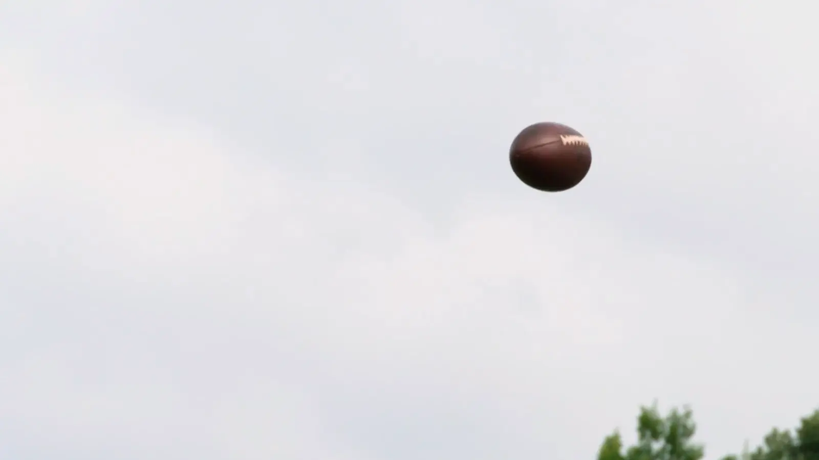
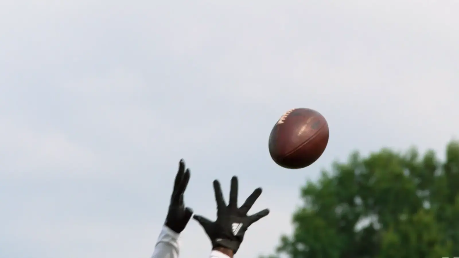
Any fan of the NFL can appreciate the beauty of a perfect spiral pass. We've seen it time and time again: a quarterback steps forward, cocks the ball back, and launches a deep pass off their fingertips. The ball points upwards immediately after release, but as the ball sails through the air, the nose gradually dips downwards before landing right in the hands of the receiver.

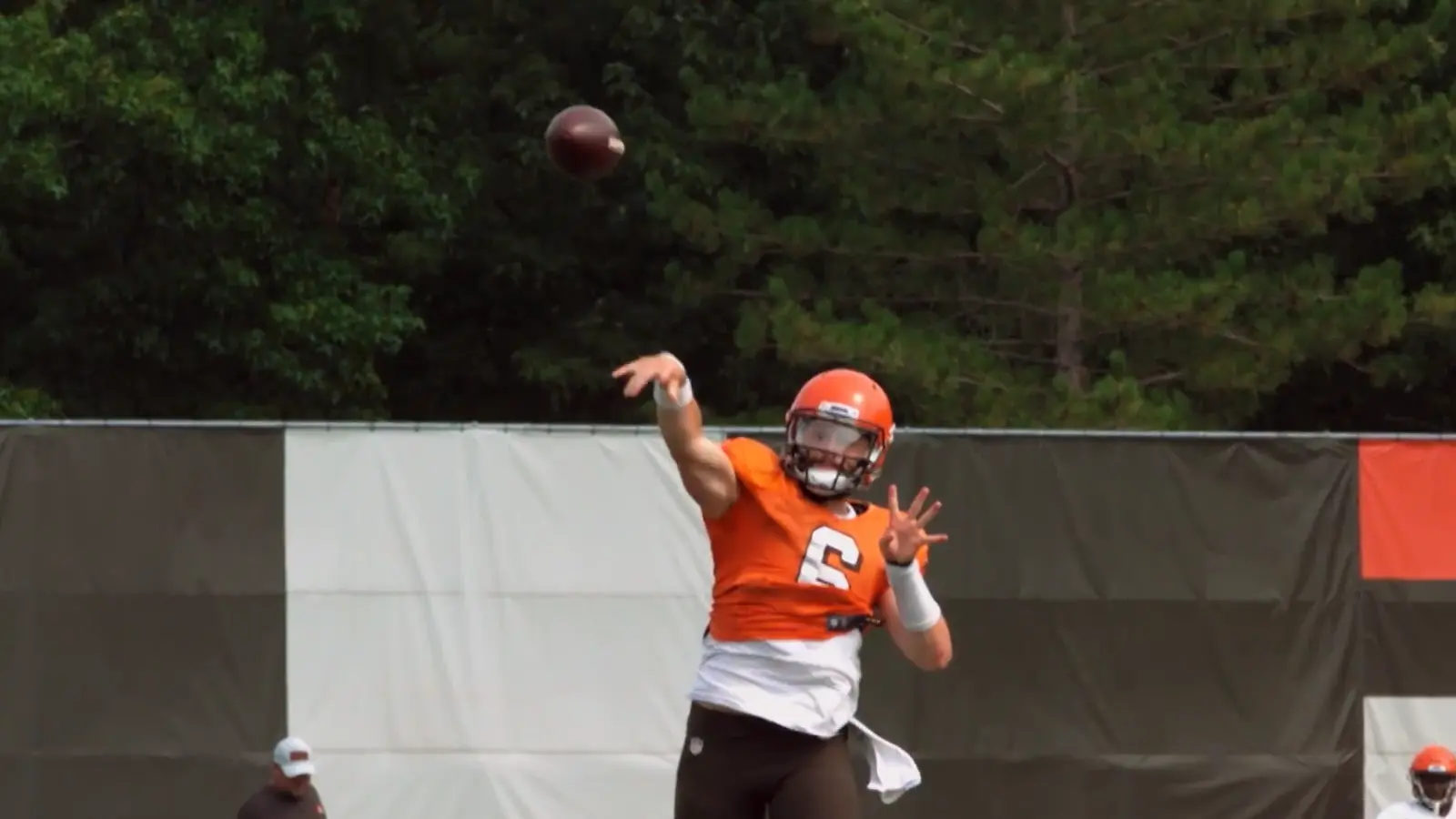
A quarterback releasing a football — The ball is released at an upwards angle.

The football at the peak of its trajectory — The ball is released at an upwards angle.

The longitudinal axis of the football remains tangent to the football's velocity throughout its flight, a quirk that football fans and players often take for granted. It makes sense that the angle of the ball would follow its trajectory to reduce drag. However, there's just one problem. The law of conservation of angular momentum in physics states that the angular momentum of an object remains constant when no net external torque acts upon it. In other words, the longitudinal axis of a spinning object maintains its orientation unless torque causes it to move. Torque is a measure of the force that causes an object to rotate. Think of a door: when you push a door open, you apply torque by rotating it around its hinges.

Conservation of angular momentum is made evident by the example of a spinning top. A spinning top continues to spin because its angular momentum points up and remains constant due to the lack of external torque affecting the top's rotation. It's important to note that the force of gravity does not cause torque, because it's applied to the center of the top and doesn't affect its rotation. Over time, though, the dissipative force of friction causes enough external torque for the top to become unbalanced and topple.

In the case of a spiraling football, there's no friction to cause torque on the ball. Gravity again acts equally on all parts of the ball, so it doesn't cause torque either. Therefore, the nose of the ball should point upwards throughout its entire arc by conservation of angular momentum. So why does it dip?

Air Resistance

If neither gravity nor friction can explain this phenomenon, there's only one possibility left: air resistance. In physics class, the effect of air resistance is often so negligible that we completely ignore it. But could it be what causes a spiraling football to orient itself with its trajectory?

When you envision a spiral, it seems as if air resistance would have the exact opposite effect: the air would push against the nose of the ball and rotate it backwards against its trajectory. We must employ a more careful mathematical approach to determine exactly how air resistance causes a perfect spiral to maintain tangency with its trajectory.

Setup

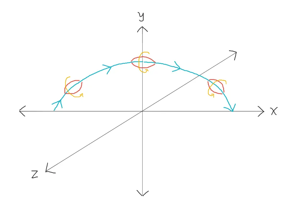
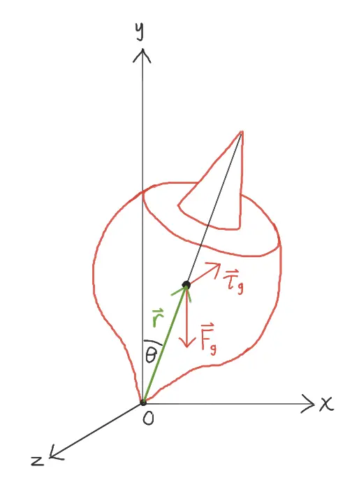
We will represent the flight of a spiral pass in $xyz$ space such that the football's trajectory begins on the negative $x$ axis, intersects the positive $y$ axis, and ends on the positive $x$ axis, as shown in #fig-geometry. The $z$ axis is perpendicular to the plane of the page.

#fig-geometry

A diagram of a coordinate plane with a football whose trajectory intersects the -x axis, the +y axis, and then the +x axis — Our chosen coordinate system geometry. The ball travels within the $xy$ plane and rotates clockwise from the perspective of the quarterback.

We must consider the ball's velocity $\mathbf{v}$ and the direction $\mathbf{\hat{d}}$ of its longitudinal axis. The spiral of the ball itself is also a factor in its flight, so we will consider the ball's angular momentum $\mathbf{L}.$

Given that the ball is thrown straight, $\mathbf{v}$ and $\mathbf{\hat{d}}$ are both vectors in the $xy$ plane. To determine the direction of $\mathbf{L},$ we use the formula

\mathbf{L} = \mathbf{r} \times \mathbf{p} \text{,}

where $\mathbf{r}$ represents the position of a point on the object relative to the center of mass, and $\mathbf{p}$ represents the linear momentum at that point. For a right-handed quarterback, the ball spirals clockwise, so we can determine using the right-hand rule that $\mathbf{L}$ also points along the $xy$ plane in the direction of $+y.$

#fig-vectors

A diagram of a football at an instant with the aforementioned vectors in 3D and 2D space — The relevant vectors in our investigation of the flight of a spiraling football.

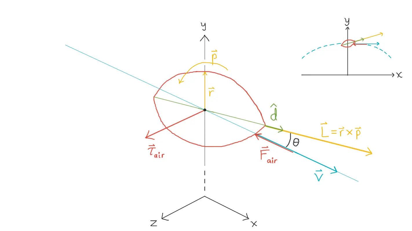
Because $\mathbf{L}$ is perpendicular to $\mathbf{r}$ and $\mathbf{r}$ is perpendicular to $\mathbf{\hat{d}}$ in the $xy$ plane, we can conclude that $\mathbf{L}$ is colinear with $\mathbf{\hat{d}},$ which means that the angle between them is $0.$ Therefore, we can set

#eq-L

\mathbf{L} = L\mathbf{\hat{d}}\text{,}

where $L$ is the magnitude of $\mathbf{L}.$

In a truly "perfect" spiral, $\mathbf{v}$ would also be colinear with $\mathbf{L}$ and $\mathbf{\hat{d}}$ ; however, this is not realistic. As shown in #fig-vectors, $\mathbf{v}$ may not be aligned with $\mathbf{\hat{d}}.$ This is the key to our problem. If you watch slow-motion video of deep balls, you will notice that every pass wobbles, even if only just a tiny bit. Not even Tom Brady can throw a perfectly tight spiral that doesn't wobble!

Why is wobble important? The force due to air resistance is given by

#eq-drag

\mathbf{F}_{\text{air}} = -\frac{1}{2}\rho AC|\mathbf{v}|^2\mathbf{\hat{v}}\text{,}

where $\rho$ is the density of air, $A$ is the cross-sectional area of the object, and $C$ is the drag coefficient of the object. #eq-drag tells us that $\mathbf{F}_{\text{air}}$ and $\mathbf{v}$ are colinear and opposite. Without wobble, $\mathbf{F}_{\text{air}}$ and $\mathbf{\hat{d}}$ would then also be colinear and opposite, so $\mathbf{F}_{\text{air}}$ should cause no torque on the ball. Indeed, we can prove this using the definition of torque

\pmb{\tau} = \mathbf{r} \times \mathbf{F}\text{.}

In our case, $\mathbf{r} = \ell\mathbf{\hat{d}},$ where $\ell$ is the length from the football's center of mass to its nose, and $\mathbf{F} = \mathbf{F}_{\text{air}}.$ Therefore,

#eq-air-torque-1

\begin{split} \pmb{\tau}_{\text{air}} &= \ell\mathbf{\hat{d}} \times \mathbf{F}_{\text{air}} \\ &= \ell \cdot -\frac{1}{2}\ell\rho AC|\mathbf{v}|^2(\mathbf{\hat{d}} \times \mathbf{\hat{v}}) \propto \sin{(\theta)} \\ &= \frac{1}{2}\ell\rho AC|\mathbf{v}|^2(\mathbf{\hat{v}} \times \mathbf{\hat{d}}) \propto \sin{(\theta)} \\ &= \kappa(\mathbf{\hat{v}} \times \mathbf{\hat{d}}) \propto \sin{(\theta)}\text{,} \end{split}

where $\theta$ is the angle between $\mathbf{\hat{d}}$ and $\mathbf{v}$ and

\kappa = \frac{1}{2}\ell\rho AC|\mathbf{v}|^2\text{.}

Note that $\pmb{\tau}_{\text{air}}$ points in the direction of the cross product of $\mathbf{\hat{v}}$ and $\mathbf{\hat{d}}.$ As shown in #fig-vectors, $\pmb{\tau}_{\text{air}}$ initially points in the positive $z$ direction due to the right-hand rule. From #eq-air-torque-1 it is easy to tell that $\pmb{\tau}_{\text{air}} = 0$ when $\theta = 0,$ or when there is no wobble.

When the ball does wobble, the direction of $\mathbf{\hat{d}}$ deviates from the direction of $\mathbf{v},$ so $\theta > 0$ and $\pmb{\tau}_{\text{air}} > 0.$ The issue, however, is that when $\theta = \pi/2,$ $\pmb{\tau}_{\text{air}} = -\kappa\mathbf{\hat{z}}$ when it should, in theory, equal $0$ because $\mathbf{F}_{\text{air}}$ would occur at the base of the ball perpendicular to $\mathbf{\hat{d}}.$ Imagine a football falling straight down with its longitudinal axis parallel to the ground; air resistance would have no effect on the ball's tilt. To resolve this, we simply halve the period of $\pmb{\tau}_{\text{air}},$ giving

#eq-air-torque-2

\pmb{\tau}_{\text{air}} = \kappa(\mathbf{\hat{v}} \times \mathbf{\hat{d}}) \propto \sin{(2\theta)}\text{.}

Now, $\pmb{\tau}_{\text{air}} = 0$ at $\theta = \pi/2$ as desired.

The angle of wobble in a well-thrown spiral is small, so we can apply the small-angle approximation $\sin{\theta}=\theta$ to #eq-air-torque-2 to produce a final equation

#eq-air-torque-3

\pmb{\tau}_{\text{air}} = 2\kappa(\mathbf{\hat{v}} \times \mathbf{\hat{d}}) \propto \theta \text{.}

Because we are primarily concerned with the behavior of $\mathbf{\hat{d}}$ in relation to $\mathbf{v},$ we assume that $\mathbf{v}$ follows a fixed parabolic path per the rules of projectile motion and is not affected by air resistance, allowing us to focus solely on $\pmb{\tau}_{\text{air}}$ and its effect.

Visualization

Before we conduct any calculations, we should first try to predict intuitively how the torque due to air resistance will affect the ball.

At the time the ball is released from the quarterback's hand, $\mathbf{\hat{d}},$ $\mathbf{L},$ and $\mathbf{v}$ are aligned. Immediately after launch, the force of gravity would cause $\mathbf{v}$ to tilt downwards, which separates it from $\mathbf{\hat{d}}$ and causes a torque in the $+z$ direction as shown in #fig-precession(a).

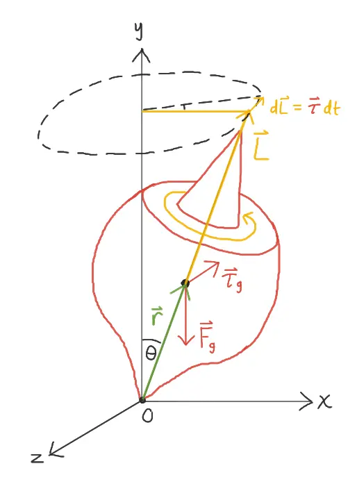
By the rotational equivalent of Newton's second law (we will use Newton's over-dot notation to denote a time derivative),

#eq-second-law

\frac{\mathbf{dL}}{dt} = \mathbf{\dot{L}} = \pmb{\tau}\text{.}

Therefore, the torque causes a change in the ball's angular momentum in the $+z$ direction. #eq-L tells us that $\mathbf{L}$ is aligned with $\mathbf{\hat{d}},$ so $\mathbf{\hat{d}}$ is also transformed in the $+z$ direction. In other words, the nose tilts to the right from the quarterback's point of view, or to the left from the receiver's point of view as shown in #fig-precession(b).

Let's quickly define a couple of terms commonly used in the field of aerospace to make this explanation easier. Yaw is the rotation of the football about its $y$ axis that changes the direction it is pointing to the left or right of its direction of velocity. Pitch is the rotation of the football about its $z$ axis that raises or lowers its nose. As such, the torque in the $+z$ direction causes the ball to "yaw right".

#fig-precession

A diagram of a football at an instant moving in the xy plane from a head-on perspective — $\mathbf{v}$ points at a higher angle than $\mathbf{\hat{d}},$ creating a torque $\pmb{\tau}$ in the $+z$ direction.

A diagram of the same football at an instant shortly after the first — $\mathbf{v}$ points at a higher angle than $\mathbf{\hat{d}},$ creating a torque $\pmb{\tau}$ in the $+z$ direction.

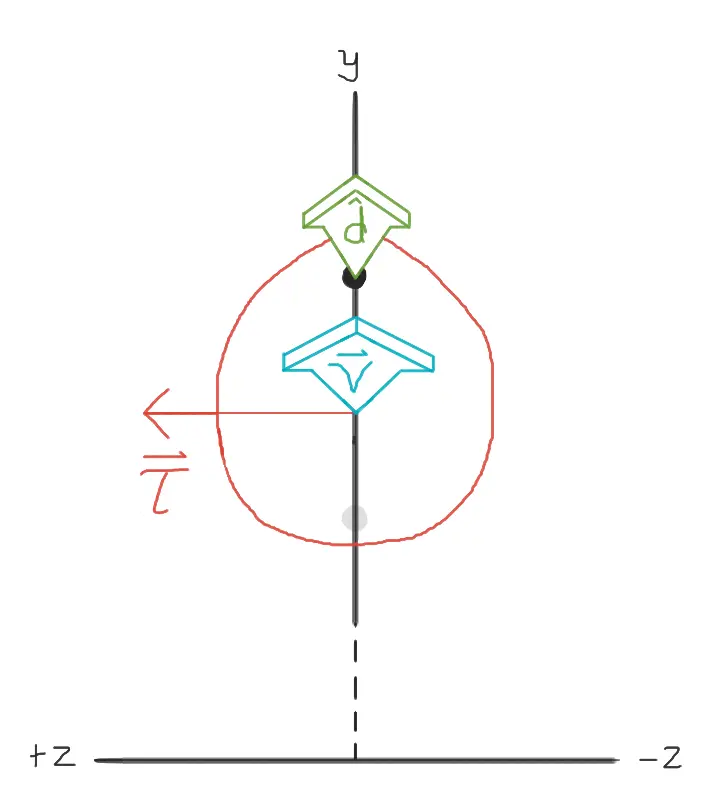
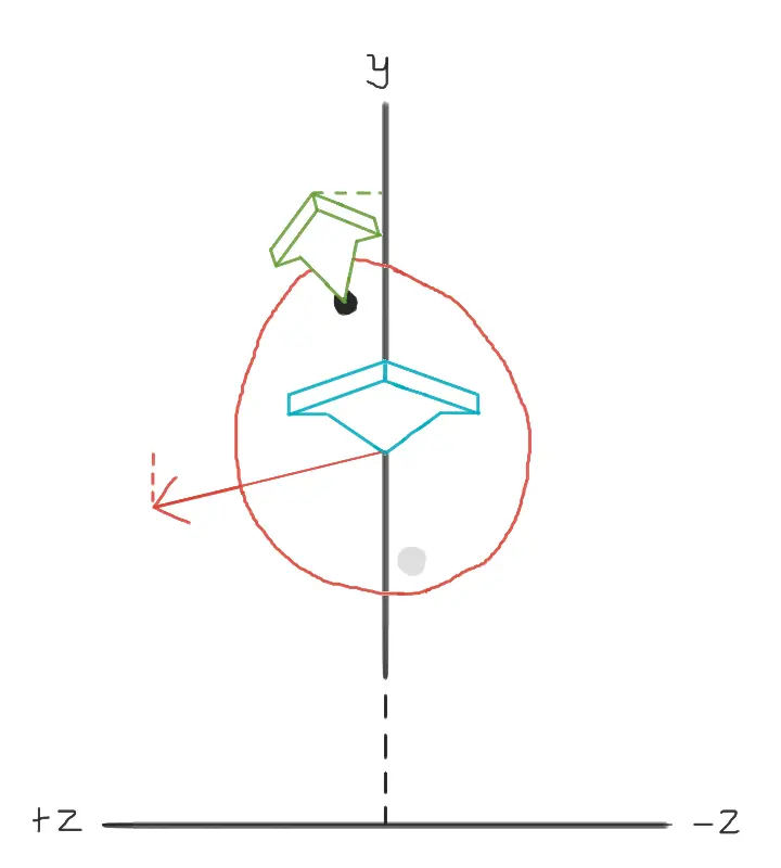
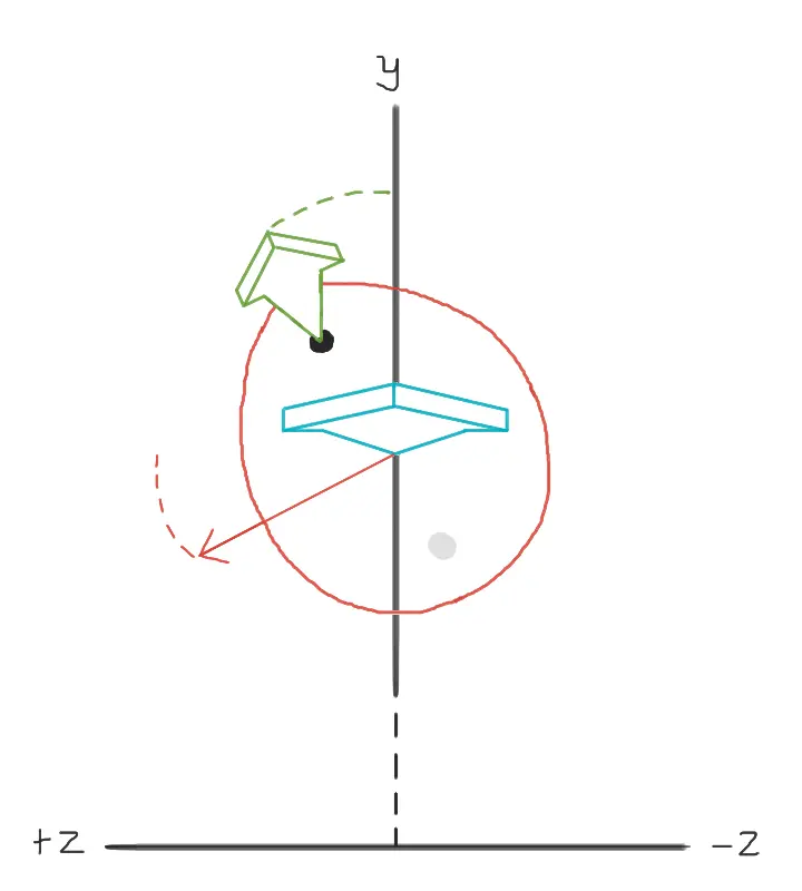
Because $\mathbf{\hat{d}}$ now has a component in the the $+z$ direction, the torque develops a component in the $-y$ direction by the right-hand rule, as shown in #fig-precession(b). Consequently, the ball pitches downwards, creating a component of torque in the $-z$ direction again by the right-hand rule, as shown in #fig-precession(c). This new torque will alter the ball's yaw, which will alter the torque, which will alter the ball's pitch, and so on. This cycle of interaction between torque and $\mathbf{\hat{d}}$ is analogous to the relationship between velocity and centripetal acceleration, so we can infer that $\mathbf{\hat{d}}$ , and equivalently the nose of the football, moves in an approximately circular path within the $yz$ plane. Indeed, this is a common behavior in spinning objects known as gyroscopic precession.

A gyroscope is a spinning object, such as a top, whose axis of rotation is free to assume any orientation. Precession is a change in the orientation of the axis of rotation. Gyroscopic precession describes how a gyroscope precesses, which we can imagine using the example of a top. If you place a top at an angle on a flat surface without spinning it, it will fall over due to the torque caused by gravity, as shown in #fig-top(a). If the top is spinning, however, it will have an angular momentum $\mathbf{L}$ pointing upwards in the axis of rotation, as shown in #fig-top(b). The torque will then cause a change in $\mathbf{L}$ according to #eq-second-law. Because the torque is always horizontal and perpendicular to $\mathbf{L}$ , the top precesses about the $y$ axis, and the tip follows the circular dotted path. In the case of a spiral pass, the torque is always perpendicular to $\mathbf{L}$ , so the nose precesses about some axis.

#fig-top

A diagram of an idle top falling over — When the top is not spinning, the torque due to gravity $\pmb{\tau_g}$ causes the top to fall over.

A diagram of a spinning top precessing about the y axis — When the top is not spinning, the torque due to gravity $\pmb{\tau_g}$ causes the top to fall over.

Gyroscopic precession explains how torque due to air resistance can affect the pitch of a spiraling football.

#fig-precession also illustrates how $\mathbf{v}$ slowly rotates downwards due to gravity throughout this flight. Knowing that $\mathbf{\hat{d}}$ maintains general tangency with the trajectory of the ball, we can predict that the ball precesses relative to $\mathbf{v}$ rather than some fixed point. Now, we must do the math to determine the exact nature in which the nose moves.

Calculations

We start by trying to find the rate $\omega_p$ at which the ball gyroscopically precesses. From #eq-air-torque-3, $|\pmb{\tau}_{\text{air}}| = \tau_{\text{air}} = 2\kappa\theta$ . Substituting into #eq-second-law and multiplying by $dt$ gives us

dL = 2\kappa\theta dt\text{.}

The radius of the dotted circle in #fig-top(b) is $L\sin{\theta}$ , which simplifies to $L\theta$ by the small-angle approximation. Thus, the angle $\phi$ that the ball precesses through in time $dt$ is

d\phi = \frac{dL}{L\theta} = \frac{2\kappa\theta}{L\theta}dt = \frac{2\kappa}{L}dt\text{.}

The angular velocity of precession would be $\frac{d\phi}{dt}$ , so we divide by $dt$ to finish with

#eq-omega

\omega_p = \frac{d\phi}{dt} = \frac{2\kappa}{L}\text{.}

We can now use #eq-omega to model the movement of $\mathbf{\hat{d}}$ over time. Substituting #eq-air-torque-3 into #eq-second-law,

#eq-L-dot

\mathbf{\dot{L}} = 2\kappa(\mathbf{\hat{v}} \times \mathbf{\hat{d}})\text{.}

$\mathbf{L} = L\mathbf{\hat{d}}$ from #eq-L so we substitute into the left-hand side to get

L\mathbf{\dot{\hat{d}}} = 2\kappa(\mathbf{\hat{v}} \times \mathbf{\hat{d}})\text{.}

We keep $L$ outside of the derivative because we know from the previous section that precession does not change the magnitude of $\mathbf{L}$ , only its direction. This allows us to divide both sides by $L$ , so #eq-L-dot becomes

#eq-d-dot

\mathbf{\dot{\hat{d}}} = \frac{2\kappa}{L}(\mathbf{\hat{v}} \times \mathbf{\hat{d}}) = \omega_p(\mathbf{\hat{v}} \times \mathbf{\hat{d}})\text{.}

Still, we are concerned not with how $\mathbf{\hat{d}}$ behaves by itself, but with how $\mathbf{\hat{d}}$ behaves relative to $\mathbf{\hat{v}}$ . To obtain insight into the manner in which $\mathbf{\hat{d}}$ deviates from $\mathbf{\hat{v}}$ , we consider the projection $\mathbf{P}$ of $\mathbf{\hat{d}}$ onto a plane perpendicular to $\mathbf{\hat{v}}$ . This plane shall be specified by the coordinate system $(\mathbf{\hat{X}}, \mathbf{\hat{Y}})$ defined by $(\mathbf{\hat{z}}, \mathbf{\hat{z}} \times \mathbf{\hat{v}})$ , as illustrated in #fig-projection. Thus, we define $\mathbf{P}$ as

\mathbf{P} = P_X \mathbf{\hat{X}} + P_Y \mathbf{\hat{Y}}\text{,}

where we can think of $P_X$ as the ball's yaw and $P_Y$ as the ball's pitch.

#fig-projection

A diagram of a football at an instant moving in the xy plane whose d-hat vector is projected upon the projection plane — An illustration of our projection plane (in yellow), made up by the $\mathbf{\hat{X}}$ and $\mathbf{\hat{Y}}$ axes. By definition, $\mathbf{\hat{X}}$ is parallel to the $z$ axis and $\mathbf{\hat{Y}}$ is perpendicular to both the $z$ axis and $\mathbf{v}$ . Vector $\mathbf{P} = \langle P_X, P_Y \rangle$ (in green) is the projection of $\mathbf{\hat{d}}$ onto our plane.

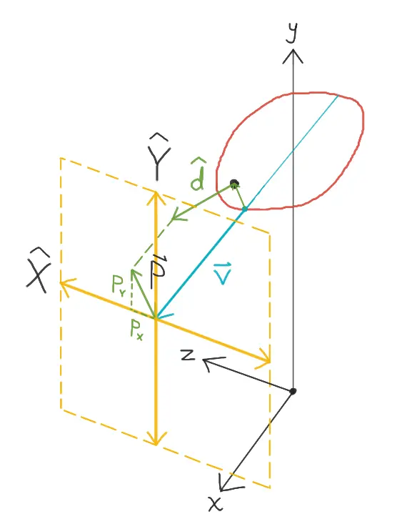
To determine $P_X$ , we must calculate the magnitude of the vector projection of $\mathbf{\hat{d}}$ onto $\mathbf{\hat{X}}$ :

#eq-P-X

\begin{split} P_X &= |proj_{\mathbf{\hat{X}}}\mathbf{\hat{d}}| \\ &= \mathbf{\hat{d}} \boldsymbol{\cdot} \mathbf{\hat{X}} \\ &= \mathbf{\hat{d}} \boldsymbol{\cdot} \mathbf{\hat{z}} \\ &= \langle \hat{d}_x,\hat{d}_y,\hat{d}_z \rangle \boldsymbol{\cdot} \langle 0,0,1 \rangle \\ &= \hat{d}_z\text{.} \end{split}

And to determine $P_Y$ , we calculate the magnitude of the vector projection of $\mathbf{\hat{d}}$ onto $\mathbf{\hat{Y}}$ :

#eq-P-Y

\begin{split} P_Y &= |proj_{\mathbf{\hat{Y}}}\mathbf{\hat{d}}| \\ &= \mathbf{\hat{d}} \boldsymbol{\cdot} \mathbf{\hat{Y}} \\ &= \mathbf{\hat{d}} \boldsymbol{\cdot} (\mathbf{\hat{z}} \times \mathbf{\hat{v}}) \\ &= \langle \hat{d}_x,\hat{d}_y,\hat{d}_z \rangle \boldsymbol{\cdot} (\langle 0,0,1 \rangle \times \langle \hat{v}_x,\hat{v}_y,\hat{v}_z \rangle) \\ &= \langle \hat{d}_x,\hat{d}_y,\hat{d}_z \rangle \boldsymbol{\cdot} \langle -\hat{v}_y,\hat{v}_x,0 \rangle \\ &= \hat{d}_y\hat{v}_x - \hat{d}_x\hat{v}_y\text{.} \end{split}

We ultimately want expressions for $P_X$ and $P_Y$ in terms of just $t$ and other constants such that we can graph our results. To do so, we first expand #eq-d-dot, resulting in

#eq-d-dot-expanded

\begin{split} \mathbf{\dot{\hat{d}}} &= \omega_p(\mathbf{\hat{v}} \times \mathbf{\hat{d}}) \\ &= \omega_p(\langle \hat{v}_x,\hat{v}_y,0 \rangle \times \langle \hat{d}_x,\hat{d}_y,\hat{d}_z \rangle) \\ &= \omega_p\langle \hat{v}_y\hat{d}_z,-\hat{v}_x\hat{d}_z,\hat{v}_x\hat{d}_y-\hat{v}_y\hat{d}_x \rangle \\ &= \langle \omega_p\hat{v}_y\hat{d}_z,-\omega_p\hat{v}_x\hat{d}_z,\omega_p(\hat{v}_x\hat{d}_y-\hat{v}_y\hat{d}_x) \rangle\text{.} \end{split}

Next, we take the derivative of #eq-P-X with respect to time, which yields

#eq-P-X-dot

\dot{P_X} = \dot{\hat{d}}_z\text{.}

Substituting the appropriate component of $\mathbf{\dot{\hat{d}}}$ that we found in #eq-d-dot-expanded,

\dot{P_X} = \omega_p(\hat{v}_x\hat{d}_y-\hat{v}_y\hat{d}_x) = \omega_pP_Y\text{.}

The process of finding $\dot{P_Y}$ begins in the same manner. We differentiate #eq-P-Y with respect to time and get

\dot{P_Y} = \hat{d}_y\dot{\hat{v}}_x + \dot{\hat{d}}_y\hat{v}_x - \hat{d}_x\dot{\hat{v}}_y - \dot{\hat{d}}_x\hat{v}_y\text{.}

Substituting the appropriate component of $\mathbf{\dot{\hat{d}}}$ that we found in #eq-d-dot-expanded,

#eq-P-Y-dot-1

\begin{split} \dot{P_Y} &= \hat{d}_y\dot{\hat{v}}_x -\omega_p\hat{v}_x\hat{d}_z\hat{v}_x - \hat{d}_x\dot{\hat{v}}_y - \omega_p\hat{v}_y\hat{d}_z\hat{v}_y \\ &= -\omega_p\hat{d}_z(\dot{\hat{v}}_x^2+\dot{\hat{v}}_y^2) + \hat{d}_y\dot{\hat{v}}_x - \hat{d}_x\dot{\hat{v}}_y \\ &= -\omega_p\hat{d}_z + \hat{d}_y\dot{\hat{v}}_x - \hat{d}_x\dot{\hat{v}}_y\text{.} \end{split}

This one's not so simple. However, we can use the fact that the football moves in a parabolic path, as illustrated in #fig-geometry, to our advantage.

If we make the assumption that $\mathbf{v}$ follows a semicircular trajectory, then we can define $\mathbf{\hat{v}}$ using the parametric unit circle equations

#eqs-v-hat

\begin{split} \hat{v}_x &= -\cos{\Omega t}\text{;} \\ \hat{v}_y &= \sin{\Omega t}\text{,} \end{split}

where $\Omega$ is the constant angular velocity of $\mathbf{\hat{v}}$ in the $xy$ plane. The path of the football under gravity is certainly more complex, but these equations shall suffice.

Our model allows us to greatly simplify #eq-P-Y-dot-1. We take the time derivatives of #eqs-v-hat and substitute for their respective components of $\mathbf{\dot{\hat{v}}}$ , giving

#eq-P-Y-dot-2

\begin{split} \dot{P_Y} &= -\omega_p\hat{d}_z + \hat{d}_y(\Omega\sin{\Omega t}) - \hat{d}_x(\Omega\cos{\Omega t}) \\ &= -\omega_p\hat{d}_z + \hat{d}_y(\Omega\hat{v}_y) + \hat{d}_x(\Omega\hat{v}_x) \\ &= -\omega_p\hat{d}_z + \Omega(\hat{d}_y\hat{v}_y + \hat{d}_x\hat{v}_x)\text{.} \end{split}

When the ball is thrown at $t=0$ , $\mathbf{\hat{d}}$ and $\mathbf{\hat{v}}$ are co-linear. Thus, the expression in parenthesis becomes

#eq-d-dot-v

\hat{d}_y\hat{v}_y + \hat{d}_x\hat{v}_x = \mathbf{\hat{d}} \boldsymbol{\cdot} \mathbf{\hat{v}} = \mathbf{\hat{v}} \boldsymbol{\cdot} \mathbf{\hat{v}} = 1\text{.}

We now combine #eq-P-Y-dot-2 with #eq-d-dot-v and #eq-P-Y to obtain

#eq-P-Y-dot-3

\dot{P_Y} = -\omega_pP_X + \Omega\text{.}

#eq-P-X-dot and #eq-P-Y-dot-3 form a system of first-order differential equations which we can write as

#eq-P-system

\mathbf{\dot{P}} = \begin{bmatrix} 0 & \omega_p \\ -\omega_p & 0 \end{bmatrix}\mathbf{P} + \begin{bmatrix} 0 \\ \Omega \end{bmatrix} = \mathbf{AP} + \mathbf{G}\text{,}

where $\mathbf{P} = \langle P_X, P_Y \rangle$ and $\mathbf{P}(0) = \langle 0, 0 \rangle$ because $\mathbf{\hat{d}}$ and $\mathbf{\hat{v}}$ are initially aligned.

To solve #eq-P-system we first consider the corresponding homogeneous system

#eq-P-system-homo

\mathbf{\dot{P}} = \mathbf{AP}, \mathbf{A} = \begin{bmatrix} 0 & \omega_p \\ -\omega_p & 0 \end{bmatrix}\text{.}

We solve #eq-P-system-homo by assuming that solutions take the form

\mathbf{P} = \pmb{\xi}e^{rt}\text{,}

where the exponent $r$ and the vector $\pmb{\xi}$ are to be determined. Substituting into #eq-P-system-homo gives

r\pmb{\xi}e^{rt} = \mathbf{A}\pmb{\xi}e^{rt}\text{,}

which we can reduce to

(\mathbf{A} - r\mathbf{I})\pmb{\xi} = \mathbf{0}\text{.}

This leads us to the system of algebraic equations

#eq-eigensystem

\begin{bmatrix} -r & \omega_p \\ -\omega_p & -r \end{bmatrix} \begin{bmatrix} \xi_1 \\ \xi_2 \end{bmatrix} = \begin{bmatrix} 0 \\ 0 \end{bmatrix}\text{.}

#eq-eigensystem has a nontrivial solution ( $\pmb{\xi} \neq \mathbf{0}$ ) if and only if the determinant of coefficients is $0$ , or equivalently, when

#eq-characteristic

\begin{vmatrix} -r & \omega_p \\ -\omega_p & -r \end{vmatrix} = r^2 + \omega_p^2 = 0\text{.}

The solutions, or eigenvalues, of #eq-characteristic are $r_1 = +\omega_p i$ and $r_2 = -\omega_p i$ . In the case of $r_1$ , #eq-eigensystem becomes

\begin{bmatrix} -\omega_p i & \omega_p \\ -\omega_p & -\omega_p i \end{bmatrix} \begin{bmatrix} \xi_1 \\ \xi_2 \end{bmatrix} = \begin{bmatrix} 0 \\ 0 \end{bmatrix} \implies \begin{bmatrix} i & -1 \\ 1 & i \end{bmatrix} \begin{bmatrix} \xi_1 \\ \xi_2 \end{bmatrix} = \begin{bmatrix} 0 \\ 0 \end{bmatrix}\text{,}

so the corresponding eigenvector

\pmb{\xi}^{(1)} = \begin{bmatrix} -i \\ 1 \end{bmatrix}\text{.}

In the case of $r_2$ , #eq-eigensystem becomes

\begin{bmatrix} \omega_p i & \omega_p \\ -\omega_p & \omega_p i \end{bmatrix} \begin{bmatrix} \xi_1 \\ \xi_2 \end{bmatrix} = \begin{bmatrix} 0 \\ 0 \end{bmatrix} \implies \begin{bmatrix} i & 1 \\ -1 & i \end{bmatrix} \begin{bmatrix} \xi_1 \\ \xi_2 \end{bmatrix} = \begin{bmatrix} 0 \\ 0 \end{bmatrix}\text{,}

so the corresponding eigenvector

\pmb{\xi}^{(2)} = \begin{bmatrix} i \\ 1 \end{bmatrix}\text{.}

Hence a fundamental set of solutions to the system described by #eq-P-system-homo is

\mathbf{P}^{(1)} = \begin{bmatrix} -i \\ 1 \end{bmatrix} e^{\omega_pit}\text{, } \mathbf{P}^{(2)} = \begin{bmatrix} i \\ 1 \end{bmatrix} e^{-\omega_pit}\text{.}

However, we want a set of real-valued solutions that we can graph. To obtain these, we choose either $\mathbf{P}^{(1)}$ or $\mathbf{P}^{(2)}$ and separate it into its real and imaginary parts. Proceeding with the former,

#eq-P-separated

\mathbf{P}^{(1)} = \begin{bmatrix} -i \\ 1 \end{bmatrix} (\cos{\omega_p t} + i\sin{\omega_p t}) = \begin{bmatrix} \sin{\omega_p t} \\ \cos{\omega_p t} \end{bmatrix} + i\begin{bmatrix} -\cos{\omega_p t} \\ \sin{\omega_p t} \end{bmatrix}\text{.}

It is easy to prove that the real and imaginary parts of any $\mathbf{P}$ form a set of solutions of #eq-P-system-homo. We simply substitute $\pmb{\Re}(\mathbf{P}) + i\pmb{\Im}(\mathbf{P})$ for $\mathbf{P}$ , obtaining

\begin{split} \mathbf{\dot{P}} - \mathbf{AP} &= \mathbf{\dot{\pmb{\Re}(P)}} + i\mathbf{\dot{\pmb{\Im}(P)}} - \mathbf{A}\pmb{\Re}(\mathbf{P}) - i\mathbf{A}\pmb{\Im}(\mathbf{P}) \\ &= (\mathbf{\dot{\pmb{\Re}(P)}} - \mathbf{A}\pmb{\Re}(\mathbf{P})) + i(\mathbf{\dot{\pmb{\Im}(P)}} - \mathbf{A}\pmb{\Im}(\mathbf{P})) = \mathbf{0}\text{.} \end{split}

It follows that $\mathbf{\dot{\pmb{\Re}(P)}} - \mathbf{A}\pmb{\Re}(\mathbf{P}) = \mathbf{0}$ and $\mathbf{\dot{\pmb{\Im}(P)}} - \mathbf{A}\pmb{\Im}(\mathbf{P}) = \mathbf{0}$ , so both $\pmb{\Re}(\mathbf{P})$ and $\pmb{\Im}(\mathbf{P})$ are solutions of #eq-P-system-homo.

Returning to $\mathbf{P}^{(1)}$ , we can now conclude from #eq-P-separated that a set of real-valued solutions of #eq-P-system-homo is

#eqs-P-system-homo-sols

\mathbf{P}_1 = \begin{bmatrix} \sin{\omega_p t} \\ \cos{\omega_p t} \end{bmatrix}\text{, } \mathbf{P}_2 = \begin{bmatrix} -\cos{\omega_p t} \\ \sin{\omega_p t} \end{bmatrix}\text{.}

We now turn back to the nonhomogeneous system described by #eq-P-system and seek a particular solution. We will employ the method of undetermined coefficients, in which we assume the form of the solution with the coefficients unspecified, and then look to determine them so as to satisfy the system.

Because $\mathbf{G}$ in #eq-P-system is a constant vector, we guess that the particular solution is a constant vector $\mathbf{A}$ . Making the substitution $\mathbf{P} = \mathbf{A}$ yields

#eq-particular

\mathbf{0} = \begin{bmatrix} 0 & \omega_p \\ -\omega_p & 0 \end{bmatrix}\mathbf{A} + \begin{bmatrix} 0 \\ \Omega \end{bmatrix} \implies \mathbf{A} = \begin{bmatrix} \Omega / \omega_p \\ 0 \end{bmatrix}\text{.}

Combining #eqs-P-system-homo-sols and #eq-particular gives us the general solution to #eq-P-system

#eq-P-system-general-sol

\mathbf{P} = c_1 \begin{bmatrix} \sin{\omega_p t} \\ \cos{\omega_p t} \end{bmatrix} + c_2 \begin{bmatrix} -\cos{\omega_p t} \\ \sin{\omega_p t} \end{bmatrix} + \begin{bmatrix} \Omega / \omega_p \\ 0 \end{bmatrix}.

Our final step is to solve for $c_1$ and $c_2$ with respect to the initial condition $\mathbf{P}(0) = \langle 0, 0 \rangle$ . At $t=0$ , #eq-P-system-general-sol becomes

\mathbf{P} = c_1 \begin{bmatrix} 0 \\ 1 \end{bmatrix} + c_2 \begin{bmatrix} -1 \\ 0 \end{bmatrix} + \begin{bmatrix} \Omega / \omega_p \\ 0 \end{bmatrix} = \begin{bmatrix} 0 \\ 0 \end{bmatrix}\text{,}

so $c_1 = 0$ and $c_2 = \Omega / \omega_p$ . Thus, the particular solution to #eq-P-system is

\mathbf{P} = \frac{\Omega}{\omega_p} \begin{bmatrix} -\cos{\omega_p t} \\ \sin{\omega_p t} \end{bmatrix} + \begin{bmatrix} \Omega / \omega_p \\ 0 \end{bmatrix}\text{,}

which means that

#eqs-P-system-particular-sols

\begin{split} P_X &= \frac{\Omega}{\omega_p}(1 - \cos{\omega_p t})\text{ and} \\ P_Y &= \frac{\Omega}{\omega_p}\sin{\omega_p t}\text{.} \end{split}

Success! #eqs-P-system-particular-sols are in terms of only $t$ and physical constants, so we can graph them and see how a tight spiral pass yaws and pitches over time.

Resolution

In order to visualize our equations, we must decide upon values for $\Omega$ and $\omega_p$ . To this end, we turn to wind-tunnel aerodynamic tests of the motion of a football conducted by William J. Rae (Rae), in which he determined that for a spiral pass with a launch angle of $30^{\circ}$ and a launch speed of $27.4$ m/s,

#eqs-empirical

\begin{split} t_\text{impact} &= 2.8\text{ s,} \\ \Omega &= 0.374\text{ rad/s,} \\ \omega_p &= 2.52\text{ rad/s.} \end{split}

Plugging these values into #eqs-P-system-particular-sols and graphing both equations against $t$ produces #fig-P-vs-time.

#fig-P-vs-time

A graph that displays yaw and pitch on the y-axis over time on the x-axis — The yaw $P_X$ and pitch $P_Y$ of a tight spiral pass as functions of time, with parameters given by #eqs-empirical and initial attitudes $P_X = 0$ and $P_Y = 0$ .

Note that the pitch of the football $P_Y$ follows a sine wave, so it periodically intersects $0$ . This is the resolution to our paradox! Because the ball always returns to zero pitch relative to its velocity, it appears to the viewer as if the orientation of the ball's longitudinal axis follows its trajectory. Thus, when the football descends, we see its nose dip as its pitch compensates for its downward velocity.

We can visualize this behavior in perhaps a more intuitive manner by graphing $P_X$ and $P_Y$ parametrically, which yields #fig-P-parametric.

#fig-P-parametric

A graph that displays yaw on the x-axis and pitch on the y-axis, creating a parametric circle — The path of the deviation vector $\mathbf{P}$ with initial attitudes $P_X = 0$ and $P_Y = 0$ .

#fig-P-parametric can be thought of as showing the yaw and pitch of the ball from the perspective of the quarterback, as opposed to #fig-projection, which shows $\mathbf{P}$ from roughly the perspective of the receiver. $\mathbf{P}$ starts at $(0, 0)$ , but proceeds clockwise following a circular path throughout the ball's flight. This confirms our theory that the ball gyroscopically precesses; in our case, the nose of the spiral is akin to the tip of the top in #fig-top-2.

Furthermore, #fig-precession introduces the idea that the greater $\mathbf{\hat{d}}$ is in the $+z$ direction, the stronger the torque on the ball in the $-y$ direction. #fig-P-parametric reflects this idea in that the greater $P_X$ is in the $\mathbf{\hat{X}}$ direction, the faster $P_Y$ decreases in the $\mathbf{\hat{Y}}$ direction due to torque, creating the clockwise path shown. It follows that because $P_X$ is always positive, the torque on the ball is often in the $-y$ direction, allowing the ball's longitudinal axis to keep up with its velocity's downward rotation.

In simplest terms, the angle of a spiraling football follows its trajectory because $P_Y$ regularly returns to $0$ .

Conclusion

Without gravity, the so-called paradox described in this article would not exist. Even when taking gravity and air resistance into account, a physicist who has never watch football would probably not predict that a spiral pass would maintain tangency with its trajectory. Physics, however, is often counterintuitive.

By causing the ball's velocity to dip, gravity sets off a chain reaction in which air resistance causes a torque on the ball, which causes the ball's angular momentum to rotate, which causes the ball to wobble, which causes the ball's longitudinal axis to dip with its velocity, creating an easier pass for the receiver. So next time you see a deep spiral touchdown pass on TV, try to spot the wobble in the slow motion replay. Without that wobble, those 6 points may not be on the board.

References

11.4 Precession of a Gyroscope | University Physics Volume 1. (n.d.). In Lumen Learning. Retrieved June 9, 2021, from https://courses.lumenlearning.com/suny-osuniversityphysics/chapter/11-3-precession-of-a-gyroscope/
Boyce, W. E., & DiPrima, R. C. (2012). Systems of First Order Linear Equations. In Elementary Differential Equations and Boundary Value Problems (10th ed., pp. 359–449). Wiley Global Education US.
Hard Knocks: Baker Slow Motion Practice. (n.d.). Retrieved June 9, 2021, from https://www.facebook.com/HardKnocksHBO/videos/hard-knocks-baker-slow-motion-practice/1891113581007661/
Price, R. H., Moss, W. C., & Gay, T. J. (2020). The paradox of the tight spiral pass in American football: A simple resolution. American Journal of Physics, 88(9), 704–710. https://doi.org/10.1119/10.0001388
Rae, W. J. (2003). Flight dynamics of an American football in a forward pass. Sports Engineering, 6(3), 149–163. https://doi.org/10.1007/BF02859892